
ch 7. Inferring a Binomial Proportion via the Metropolis Algorithm
30 Oct 2017 | ml bayesian inference mcmc호객행위
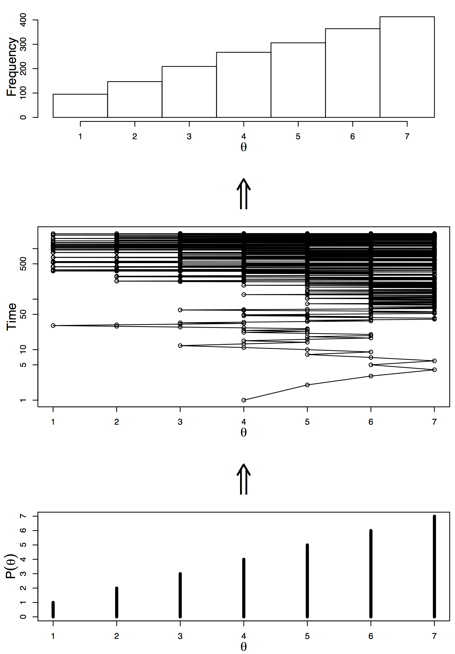
d3를 가지고 만들어본 예제이다. 왼쪽이 실제 distribution이며, 오른쪽이 sampling을 한 결과이며, burn-in은 따로 하지 않았다.
population
markov-chain
sampled
Intro
- 우리가 원하는건 posterior $p(\theta \vert D)$
- 근데 항상 evidence가 marginalize하기 쉽지 않다.
- Ch 5에서는 likelihood의 conjugate prior를 찾아서 posterior를 구했음
- Ch 6는 그냥 prior를 discrete하게 쪼개놓고 구했음 (굳이 정리를 하지 않았음)
- 잘게 쪼개면 더 정확해진다
- Ch 6는 좋은 방법이지만 parameter가 많아지면 어떡할랭?
- 1000개씩 6개의 파라미터면 $1000^6$이 돼버림..
- posterior와 비례하는 어떤 함수를 가지고있고, 계산할 수 있으면
- 많은 수의 random value들로 시뮬레이션해서 posterior distribution을 근사시켜보자!
Metropolis algorithm
예제
- 정치인이 여러 섬들을 다니면서 유세를 할 것이다.
- 섬은 총 7개가 있으며, 각 섬마다 인구 수는 다르다.
- 정치인은
- 현재 섬에 머무를지,
- 서쪽 섬으로 갈지,
- 동쪽 섬으로 갈지 판단해야한다.
- 지금 섬의 인구와, 다음에 갈 섬으로 제안된 곳의 인구 수만 알 수있다.
algorithm
- proposal distribution
- 동전을 던져 왼쪽으로 갈지, 오른쪽으로 갈지 정한다
- 한쪽이 나왔다면
- 한 쪽의 인구수가 더 많으면 무조건 이동
- 아니라면 $P_{move} = P_{proposed} / P_{current}$의 확률로 감
근데 이게 먹힌다.
결과
알아야할 것들
- burn-in
- 앞의 몇 스텝은 초기값에 따른 bias가 있으니 없앰
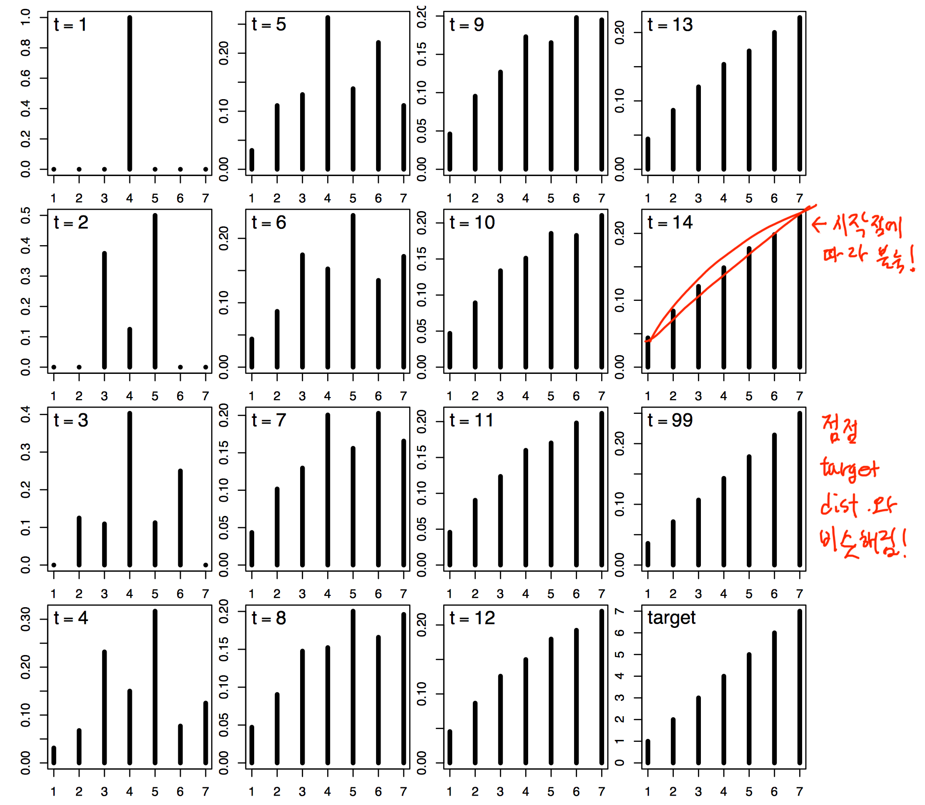
- proposal distribution을 잘 선택해야함
- narrow하면 수렴에 엄청 오래걸릴 것이다
- 초기값이 심지어 target distribution이 flat하고 low한 곳이면 수렴이 힘들지..
근데 이게 여태 하던 posterior 추정이랑 뭔 상관?
- Metropolis algorithm을 다시 한번 보면
- 이동할 확률을 $\frac{P_{proposed}}{P_{current}}$로 구함
- 즉 $P$가 normalized돼있지 않아도 됨!
- $P = p(D\vert \theta)p(\theta)$로도 충분
- 그래서 posterior를 추정할 때 좋지!
코드로 풀어보자!
동전던지기의 예제를 들어본다. $\theta$는 앞면이 나올 확률을 의미하는 parameter이다.
가정
- Prior
- $p(\theta): uniform(0,1)$
- Likelihood
- $p(z,N\vert \theta): \theta^{z}(1-\theta)^{(N-a)}$
- data
- 14번 던져서 11번이 앞면이 나옴.
Proposal distribution
$N(0, 0.2)$로 하며, 부적절한 $\theta$에 대해서는 prior나 likelihood가 0을 주면 된다.
import numpy as np
%matplotlib inline
import matplotlib.pyplot as plt

def prior(theta):
    '''
    theta에 대한 prior 확률을 return
    '''
    if theta < 0 or theta > 1:  # 여기서 처리해주자!
        return 0
    else:
        return 1

def likelihood(z, N, theta):
    '''
    theta가 주어졌을 때, z,N에 대해서 likelihood 확률을 return
    '''
    return (theta ** z)*((1-theta)**(N-z))

def proposal_dist(n):
    '''
    proposal distribution에서 n개 뽑아온다.
    '''
    return np.random.randn(n) * 0.2  # sigma는 0.2로...
N = 10000
burn_in = int(0.1*N)
theta_sampled = [0.5]

for i in range(N):
    theta = theta_sampled[-1]
    new_sample = proposal_dist(1)
    proposed_theta = theta + new_sample

    # p(D\vert ∂)p(∂) 구하기
    h1 = prior(theta) * likelihood(11, 14, theta)
    h2 = prior(proposed_theta) * likelihood(11, 14, proposed_theta)

    if h2 > h1:  # 만약 proposed가 더 확률이 크면
        theta_sampled.append(proposed_theta)
    else:  # 아니면
        s = np.random.uniform(0, 1, 1)
        if s[0] < h2/h1:
            theta_sampled.append(proposed_theta)
        else:
            theta_sampled.append(theta)


theta_sampled = theta_sampled[burn_in:]  # 처음 나온 애들은 버려야지..
plt.hist(np.array(theta_sampled), bins=50)
plt.show()
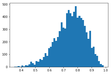 결과를 보면 잘 나오는 것을 알 수 있다.