
03.RNN 구현
13 Jan 2017 | RNN nn01. softmax classifier와 neural network 구현
NN의 다양한 구현체들 예제
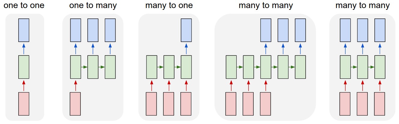
- RNN 없는 그냥 NN. 고정된 input, output size를 가진다.
- Sequence output (예> image captioning: input은 image 한장이고 output은 word들이 있는 문장)
- Sequence input (예> sentiment analysis: sentence를 input으로 하고 positive인지, negative인지 구분짓는 것)
- Sequence I/O (예> machine translation : RNN이 영어 문장을 읽고, 프랑스어로 output 문장을 낸다.)
- Synced sequence I/O (예> video classification: 각 프레임에 label을 붙이고 싶음)
RNN Computation
RNN은 그저 input x를 받아서 output y를 return하는 함수이다. 그런데 y를 내는데에 있어서 현재 넣은 input뿐만이 아니라, 과거의 input또한 영향을 미친다.
RNN class를 만든다면, step이라는 함수는 x를 받아 y를 낸다.
rnn = RNN()
y = rnn.step(x) # x is an input vector, y is the RNN's output vector
RNN은 매 step마다 업데이트되는 internal state를 가진다. 가장 단순한 것으론 vector h하나를 state로 갖는다. 다음 것은 RNN의 가장 단순한 구현이다.
class RNN:
    # ...
    def step(self, x):
        # update the hidden state
        self.h = np.tanh(np.dot(self.W_hh, self.h) + np.dot(self.W_xh, x))
        # compute the output vector
        y = np.dot(self.W_hy, self.h)
        return y
위는 vanila RNN의 forward pass를 구현한 것이다.
self.h는 0으로 초기화하며 나머지 matrix는 random하게 초기화한다. RNN에서 hidden state를 구하는 식은 다음과 같다.
이후 hidden state로 output을 구하는데 식은 다음과 같다.
Going Deep
더 딥하게 쌓으려면 단순히 다음처럼 하면 된다.
y1 = rnn1.step(x)
y = rnn2.step(y1)
이제 코드를 짜보자!
loss와 다음 state에 대한 gradient를 가지고있다는 것을 생각해보자.
def lossFun(inputs, targets, hprev):
    xs, hs, ys, ps = {}, {}, {}, {}
    hs[-1] = np.copy(hprev)
    loss = 0
    # forward pass
    for t in xrange(len(inputs)):
        xs[t] = np.zeros((vocab_size,1)) # encode in 1-of-k representation
        xs[t][inputs[t]] = 1
        hs[t] = np.tanh(np.dot(Wxh, xs[t]) + np.dot(Whh, hs[t-1]) + bh) # hidden state
        ys[t] = np.dot(Why, hs[t]) + by # unnormalized log probabilities for next chars
        ps[t] = np.exp(ys[t]) / np.sum(np.exp(ys[t])) # probabilities for next chars
        loss += -np.log(ps[t][targets[t],0]) # softmax (cross-entropy loss)
    # backward pass: compute gradients going backwards
    dWxh, dWhh, dWhy = np.zeros_like(Wxh), np.zeros_like(Whh), np.zeros_like(Why)
    dbh, dby = np.zeros_like(bh), np.zeros_like(by)
    dhnext = np.zeros_like(hs[0])
    # gradient는 역으로 계산한다. (당연히 backpropagation이니까)
    for t in reversed(xrange(len(inputs))):
        # dscore for loss
        dy = np.copy(ps[t])
        dy[targets[t]] -= 1
        # 나머지...
        dWhy += np.dot(dy, hs[t].T)
        dby += dy
        #loss말고 전의 state에서 발생한 gradient를 더해준다.
        dh = np.dot(Why.T, dy) + dhnext # backprop into h
        # 또 나머지...
        dhraw = (1 - hs[t] * hs[t]) * dh # backprop through tanh nonlinearity (tanh' = 1-tanh^2)
        dbh += dhraw
        dWxh += np.dot(dhraw, xs[t].T)
        dWhh += np.dot(dhraw, hs[t-1].T)
        dhnext = np.dot(Whh.T, dhraw)  # hs[t-1]에 대한 미분값

    for dparam in [dWxh, dWhh, dWhy, dbh, dby]:
        np.clip(dparam, -5, 5, out=dparam) # clip to mitigate exploding gradients
    return loss, dWxh, dWhh, dWhy, dbh, dby, hs[len(inputs)-1]