image resizing

13 Nov 2017 | numpy scipy imageio

%matplotlib inline
import matplotlib.pyplot as plt
import numpy as np
import imageio
import scipy.misc

im = imageio.imread('test.jpg')  # 읽고
plt.imshow(im)
print(im.shape)

(1044, 1179, 3)

i_width = 32
i_height = 32

im2 = scipy.misc.imresize(im, (i_height, i_width))  # resize

plt.imshow(im2)
print(im2.shape)

(32, 32, 3)

im2 = im2.astype(np.float32)
im2 = im2/255.0

tensorflow에서 image batch로 만들어 보내는 예제..

13 Nov 2017 | batch image tensorflow

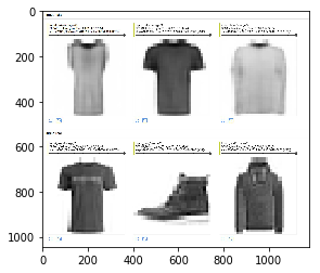
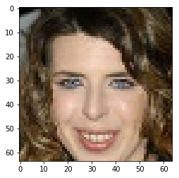
CelebA Image batch로…

%matplotlib inline
import matplotlib.pyplot as plt
import numpy as np
import imageio
import tensorflow as tf

import os
os.environ["CUDA_DEVICE_ORDER"]="PCI_BUS_ID"
os.environ["CUDA_VISIBLE_DEVICES"]="7"

def batch(file_list, batch_size=16):
    fileQ = tf.train.string_input_producer(file_list, shuffle=False)
    reader = tf.WholeFileReader()

    filename, data = reader.read(fileQ)
    image = tf.image.decode_jpeg(data, channels=3)

    img = imageio.imread(file_list[0])
    w, h, c = img.shape
    shape = [w, h, 3]
    
    image.set_shape(shape)
    min_after_dequeue = 10000
    capacity = min_after_dequeue + 3 * batch_size

    queue = tf.train.shuffle_batch(
        [image], batch_size=batch_size,
        num_threads=4, capacity=capacity,
        min_after_dequeue=min_after_dequeue, name='synthetic_inputs')
    
    crop_queue = tf.image.crop_to_bounding_box(queue, 50, 25, 128, 128)
    resized = tf.image.resize_nearest_neighbor(crop_queue, [64, 64])

    return tf.to_float(resized)

import os
dir_ = '/root/CelebA/images'
jpgs = os.listdir(dir_)
filelist = [os.path.join(dir_, jpg) for jpg in jpgs]
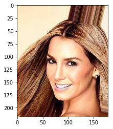
plt.imshow(imageio.imread(filelist[0]))

<matplotlib.image.AxesImage at 0x7f95ae746d68>

data_loader = batch(filelist)

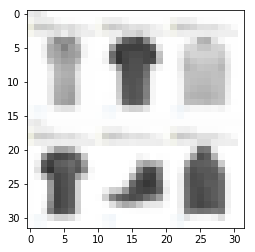
위까지 하면 batch가 만들어지고.. 한번 뽑아보자!

with tf.Session() as sess:
    sess.run(tf.global_variables_initializer())
    
    coord = tf.train.Coordinator()
    threads = tf.train.start_queue_runners(sess=sess, coord=coord)

    im = sess.run(data_loader)
    
    coord.request_stop()
    coord.join(threads)

im = im.astype(np.uint8)
plt.imshow(im[8, :])

<matplotlib.image.AxesImage at 0x7f95ac1a75f8>

표본의 분산을 구할 때 n-1하는 이유

05 Nov 2017 | statistic math

$S^2$ : sample의 분산
$\bar{X}$ : sample의 평균
$\mu$ : 실제 평균
$\sigma$ : 실제 분산

proof

GAN

02 Nov 2017 | ml generative model

참고 1

생김새

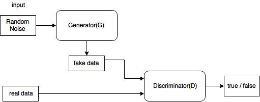요래 생겼다.

푸는 문제

$\underset{G}{min}\ \underset{D}{max} V(D, G)$

where

$V(D, G) = \textbf{E}_{x \sim p_{data}(x)}[logD(x)] + \textbf{E}_{z \sim p_{z}(z)}[log(1-D(G(z)))] -- (1)$

D 관점에서 (1)의 앞 뒤의 수식을 따로 생각해보면

Ex∼pdata(x)[logD(x)]
- data에서 나온 x(real data)는 값을 크게하고
Ez∼pz(z)[log(1−D(G(z)))]
- $p_z$ 를 통해 나온 $z$ 가 Generator를 거쳐 나온 G(z)(fake data)는 값을 작게해야

V(D, G)를 크게할 수 있다.

이제 G 관점에서 (1)의 뒷 수식만 보면

Ez∼pz(z)[log(1−D(G(z)))]
- 이걸 minimize하려면 $G(z)$ 가 최대한 x의 분포에 가깝게 가야한다.

논문에 있는 그림인데,

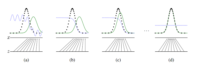
검은색: data distribution
초록색: generator distribution
파란색: discrimimnator distribution

실용적인 수식 변환

사실 (1)에서 $log(1-D(G(z)))$ 를 minimize하는 대신 $log(D(G(z)))$ 를 maximize 한다. 처음에 G가 너무 구려서 Discriminator가 구분을 잘함. 그래서 $log(1-D(G(z)))$ 에 대한 gradient가 0에 가까움.. 근데 $log(D(G(z)))$ 는 괜찮음.

이론

제안 1.

G가 고정되어있으면 최적의 discriminator D는

$D^*_G(x) = \frac{p_{data}(x)}{p_{data}(x) + p_{g}(x)}$

증명 >

일단 이것부터 증명하자. $\forall (a, b) \in \textbf{R}^2 - {(0, 0)}$ 에 대해 어떤 함수 $y \rightarrow a\cdot log(y) + b\cdot log(1-y)$ 가 존재한다면 [0, 1]사이에서 f(y)가 최대가 되는 y는 $\frac{a}{a+b}$ .

미분해서 0이되는 y를 찾으면 당연히 저 값이 나온다. 로그 두개를 하나는 반대로 만들어서 더한 꼴인데, 볼록한 형태일테고… 쉬우니까 넘어가자.

1을 증명했으면 이제 $V(D,G)$ 를 전개해보자

$\begin{align*} V(D, G) &= \int p_{data}(x)\cdot logD(x)\ dx + \int p_{z}(z)\cdot log(1-D(G(z)))\ dz \\ &= \int p_{data}(x)\cdot logD(x)\ + p_{g}(x)\cdot log(1-D(x))\ dx \end{align*}$

인데 제안 1을 사용하면 증명 끝이지?

위의 제안으로부터 $\underset{ D}{max} V(D, G)$ 는 다음처럼 바뀐다.

$\begin{align} C(G) & = \max_D V(G,D) \\ &= \mathbb{E}_{x \sim p_{data}} \left[ log D^*_G(x) \right] + \mathbb{E}_{z\sim p_z}\left[ log(1-D^*_G(G(z))) \right] \\ &= \mathbb{E}_{x \sim p_{data}} \left[ log D^*_G(x) \right] + \mathbb{E}_{x\sim p_g}\left[ log(1-D^*_G(x)) \right] \\ &= \mathbb{E}_{x \sim p_{data}} \left[ log \frac{p_{data}~(x)}{p_{data}~(x)+p_{g}(x)} \right] + \mathbb{E}_{x\sim p_g} \left[ log \frac{p_{g}(x)}{p_{data}~(x)+p_{g}(x)} \right] \end{align}$

Thorem 1.

$C(G)$ 의 global minimum이 달성 <=> $p_g = p_{data}$ . 그리고 그 때 $C(G)$ 의 값은 $-log(4)$

증명>

$p_g = p_{data}$ 일 때 C(G)값 증명

$p_g = p_{data}$ 면 $D^*_G(x)=\frac{1}{2}$ 는 당연하고.. 이를 $C(G)$ 에 넣어보면

$C(G) = \mathbb{E}_{x \sim p_{data}} \left[ -log(2)\right] + \mathbb{E}_{x \sim p_{g}} \left[ -log(2)\right]=-log(4)$

(<=>)증명 $\begin{align*}C(G) &= C(G) + log(4) -log(4) \\ &= -log(4) + \mathbb{E}_{x \sim p_{data}} \left[ log \frac{p_{data}~(x)}{p_{data}~(x)+p_{g}(x)} \right] + \mathbb{E}_{z\sim p_x(z)} \left[ log \frac{p_{g}(x)}{p_{data}~(x)+p_{g}(x)} \right] + log(2) + log(2) \\ &= -log(4) + KL \left( p_{data} \vert\vert \frac{p_{data}~+ p_g}{2}\right) + KL \left( p_g\vert\vert \frac{p_{data}~+ p_g}{2}\right) \\ &= -log(4) + 2\cdot JSD(p_{data}\vert\vert p_g) \end{align*}$ 이제 KL이나 JSD가 >=0 이니까 최저값은 -log(4)이고 그 때 $p_{data} = p_g$

두번째서 세번째 넘어가는것만 보이자 $\begin{align} \mathbb{E}_{x \sim p_{data}} \left[ log \frac{p_{data}~(x)}{p_{data}~(x)+p_{g}(x)} \right] + log(2) &= \mathbb{E}_{x \sim p_{data}} \left[ log \frac{p_{data}~(x)}{p_{data}~(x)+p_{g}(x)} + log(2) \right] \\ &= \mathbb{E}_{x \sim p_{data}} \left[ log \frac{2\cdot p_{data}~(x)}{p_{data}~(x)+p_{g}(x)} \right] \\ &= KL \left( p_{data} \vert\vert \frac{p_{data}~+ p_g}{2}\right) \end{align}$

이제 남은 건 G, D가 충분한 capacity일 때 GAN 알고리즘이 $p_g = p_{data}$ 를 achieve 하는가 증명인데…. 이건 패스

ch 8. Inferring Two Binomial Proportions via Gibbs Sampling

01 Nov 2017 | ml bayesian inference mcmc

2 Binomial이 독립인 사건에 대해서 analytic하게 풀기

$\theta_1, \theta_2$ 가 각각 다른 동전이 앞면이 나올 확률을 의미한다고 가정해보자.
그렇다면 likelihood는 다음처럼 정의된다.
- $p(D\vert \theta_1, \theta_2) = \theta_1^{z_1}(1-\theta_1)^{(N_1-z_1)}\cdot\theta_2^{z_2}(1-\theta_2)^{(N_2-z_2)}$
또한 posterior는
p(\theta_1, \theta_2 \vert D) = p(D\vert \theta_1, \theta_2)p(\theta_1, \theta_2)/ \left [ \int\int p(D\vert \theta_1, \theta_2)p(\theta_1, \theta_2)d\theta_1d\theta_2 \right ]
- 요기서 두 $\theta$ 가 독립이라고 하면 ch 5에서 본 beta distibution을 사용해서 또 analytic하게 풀 수 있다.
$\begin{align*} p(\theta_1, \theta_2 \vert D) &= p(D\vert \theta_1, \theta_2)p(\theta_1, \theta_2)/ p(D) \\ &= \frac{\theta_1^{z_1+a_1-1}(1-\theta_1)^{(N_1-z_1+b_1-1)}\cdot\theta_2^{z_2+a_2-1}(1-\theta_2)^{(N_2-z_2+b_2-1)}}{p(D)\cdot B(a_1,b_1)\cdot B(a_2,b_2)} \end{align*}$
정리하면 $p(D) = \frac{B(z_1+a_1, N_1-z_1+b_1)\cdot B(z_2+a_2, N_2-z_2+b_2)}{B(a_1,b_1)\cdot B(a_2,b_2)}$ 가 나온다.

approximation -> Gibbs

parameter space가 작을 때는 grid approximation이 좋은 대안이다.
- 어떤 prior distribution도 쓸 수 있다.
- 어떤 posterior에서 HDI 구할 때도 편하다.
하지만 parameter가 넓을 경우는 힘들어진다.
- 그럼 7장의 Metropolis algorithm을 쓰면?
- proposal dist.의 디자인에 따라서 local region에 계속 머물수도 있다.
Gibbs sampling을 소개해보자

Gibbs sampling

proposal distribution같은거 없음!
대신 나머지 파라미터가 주어진 posterior dist.에서 sampling이 가능해야함(더 빡셈)
- 즉 \theta_1, \theta_2, \theta_3이 parameter라고 하면
  - $p(\theta_1\vert \theta_2, \theta_3, D)$
  - $p(\theta_2\vert \theta_1, \theta_3, D)$
  - $p(\theta_3\vert \theta_1, \theta_2, D)$
- 에서 모두 sampling이 가능해야함.
엄청 빡센데, 요건만 만족하면 Metropolis algorithm보다 훨씬 reliable하다.
이 놈 역시 MCMC process
- 현재 position에서만 다음 스텝이 결정되고,
- sampling을 통해 simulation하니까
보통은 순서를 정해서 파라미터를 순회하면서 sample한다.
- parameter가 많아지면 random하게 파라미터를 뽑을 시, 다 뽑는데 시간이 걸림
Gibbs sampling은 Metropolis에서 proposal distribution이 지금 뽑을 parameter에 의존하는 것이라고 볼 수 있다고 한다. (이 부분 좀 잘 모르겠다..)
- 이 경우 proposal distribution이 항상 그 파라미터의 posterior probability를 반영해서, proposal이 항상 accept된다.

여기까지 보고 다시 위의 2 Binomial 예제를 Gibbs sampling으로 풀어보자!

사실 위의 예제는 너무 단순하긴한데… 그대신 쉬우니까…

\theta_1에 대한 posterior는
- $\begin{align*} p(\theta_1\vert \theta_2, D) &= p(\theta_1\vert D) \\ &= beta(\theta_1\vert z_1+a_1, N_1-z_1+b_1) \end{align*}$
요걸 가지고 실험을 해보자!

Gibbs Sampling 예제

동전던지기의 예제를 들어본다. $\theta_n$ 은 n번째 동전이 앞면이 나올 확률을 의미하는 parameter이며, 동전은 2개이다.

가정

Prior
- $p(\theta_n): beta(\theta \vert 3,3)$
Likelihood
- $p(z_n,N_n \vert \theta_n): {\theta_n}^{z_n}(1-{\theta_n})^{(N_n-z_n)}$
data
- 동전 1 - 7번 던져서 5번 앞면
- 동전 2 - 7번 던져서 2번 앞면

%matplotlib inline
import numpy as np
import matplotlib.pyplot as plt

data = [{'N': 7, 'z': 5},
        {'N': 7, 'z': 2}]

def posterior(N, z, a, b):
    return np.random.beta(z + a,
                          N - z + b)
thetas = [[0.2, 0.5]]
for i in range(100000):
    idx = i % 2
    theta = thetas[-1].copy()
    theta[idx] = posterior(data[idx]['N'],
                           data[idx]['z'],
                           3,
                           3)  # prior가 좀 세다. 1로 바꾸면 좀 더 data와 비슷하게 나옴을 알 수있다.
    thetas.append(theta)

thetas = thetas[int(len(thetas)*0.1):]  #burn-in
    

np_thetas = np.array(thetas)
x = np_thetas[:,0]
y = np_thetas[:,1]
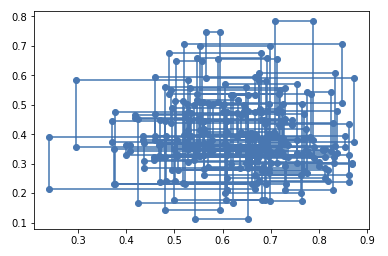
plt.plot(x[:300], y[:300], '-o')
plt.show()

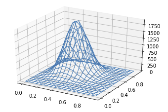
from mpl_toolkits.mplot3d import Axes3D
import matplotlib.pyplot as plt

fig = plt.figure()
ax = fig.add_subplot(111, projection='3d')

hist, xedges, yedges = np.histogram2d(x, y, bins=20, range=[[0, 1], [0, 1]])

xedges, yedges = np.meshgrid(xedges, yedges)

surf = ax.plot_wireframe(xedges[:-1,:-1],
                         yedges[:-1,:-1],
                         hist,
                         linewidth=1)

Gibbs sampling의 단점

각 파라미터의 conditional probability가 필요!
연관도가 높은 파라미터들에 대해서 progress가 멈출 수 있음
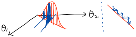- $\theta_1$ 과 $\theta_2$ 가 Highly correlated 면 왼쪽과 같은 그림이 되겠다. 이 때, 파라미터 업데이트는 오른쪽처럼 아주 작게 움직이겠다.

Older Newer

Hulk의 개인 공부용 블로그